Instrument Testing

  1. JFET Checks
    1. Summary
    2. Technique
    3. Instructions
  2. Optical Efficiency and Dewar Loading
    1. Summary
    2. Optical Setup
    3. JFETs
    4. Temperature Control Setup
    5. Bias Board Settings
    6. Cabling and DAS Setup
    7. Data-Taking Procedure
    8. Analysis Procedure
  3. Electronics Noise Testing
    1. Setup
    2. Analysis
  4. Revision History
Back to BolocamWebPage
Back to ExpertManual


JFET Checks

Summary

It is possible to check the basic operation of the JFETs and the connections of all the bolometers by the following series of tests.  These tests have become standard practice whenever the dewar is opened and reclosed.  It certainly does not hurt to do them even if the dewar has not been opened.  In the future, it is likely that we will stop doing these tests except when the dewar is opened and closed, as we now have a sufficient baseline to see that the cold electronics are not exhibiting more failures with time -- the current set of JFETs have been in place since January, 2003, and no new failures have been seen, and the current cryogenic cabling has been in place since summer, 2003, with no new failures seen.

Technique

We do these checks by simply measuring the JFET output voltages at three different bolometer biases: 0V, +40 mV asymmetric, and -40 mV asymmetric.  By "asymmetric", we mean that we use clips to tie one of the sides of the bias to 0V so that only the other side moves.  This is best illustrated by a diagram of the bolometer bias and readout:


When B+ and B- are set to 0V, the voltages we see at V+ and V- are just the JFET offset voltages, which should be well matched (within 10-20 mV of each other).

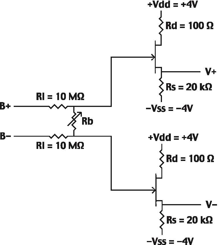
During normal operation, B+ and B- are set to equal and opposite values.  If Rb is nonzero, equal and opposite voltage appear its two ends.  The JFETs, acting as following, communicate this signal to their outputs, so V+ and V- move up and down by equal but opposite amounts, respectively.  The signal we read is the difference between the two.

When the bolometers are warm, Rb ~ 0Ω and no change will be seen in V+ and V- if B+ and B- are varied in a symmetric fashion.  However, by tying B+ or B- to zero and varying the other to some voltage Vb, the bolometer and the JFET gats move up by Vb/2.  We expect both JFET output voltages V+ and V- to increase (or decrease) by equal and same-signed amounts.

Thus, using asymmetric biasing, we can test whether the JFETs are working and the bolometer is connected even when Rb = 0.  We cannot distinguish short-circuited bolometers from working bolometers, but all other failure modes -- open-circuit bolometers, non-functional JFETs, or broken JFET output lines -- are visible.

Instructions

Do the test as follows.  It is easiest to do all three bias settings for each hextant and then cycle through hextants.
  1. You will need to monitor the bias being sent into the dewar. To do so, connect clip leads from pins 1 (B-) and 2 (B+) of the AD624 chip on the bias board corresponding to the hextant you want to check and connect to a DMM.  There are six such bias monitor circuits on the board; they should be labelled "1", "2", and so on. The AD624s should be obvious from their gold-plated packages.  The chips of interest are in the top half of the board.

  2. You will need to alternately ground the + and - sides of the bolometer bias in order to send an asymmetric bias into the dewar.  This is done by attaching clip leads from the board ground to either the B+ or B- bolometer bias lines. It is easiest to do this, and least likely to cause damage, by attaching a chip clip to the AD624 for the hextant bias monitor and grounding either pin 2 (B+) or pin 1 (B-).

  3. You will need to measure the voltages of all the JFET source lines relative to ground (V+ and V- in the above picture). We normally do this by connecting the cable G DB50 connector of the hextant of interest to a breakout box that converts from DB50 to 25 isolated BNCs (you may want to use a DB50M-DB50F extension cable so you put the breakout box in a convenient place).  Each source line pair goes to one BNC (center conductor and shield) and pins 1 and 34 go to the 25th BNC.

  4. Put the bias board into adjustable DC bias mode; see the Electronics page for instructions.

  5. To do the bias = 0 V measurement, set the bolometer bias to 0 using the front panel knobs and ground B-. It may not seem necessary to ground B- for the 0V measurement, but it is necessary because voltage offsets appear when one side of the bias is grounded.

  6. Measure the voltages at all the source lines with respect to ground. These voltages are called the "JFET offsets" -- these are the source line output voltages when the gates are at 0V.  Source lines that read out the same bolometer should have offset voltages within 10 mV of each other because the JFETs are on the same die. If the voltages are much larger than 10 mV apart, then either the JFET is problematic or you have a measurement problem. Record all the source line voltages. There is a checkout sheet available for recording these voltages: ps, pdf.  (Print out 6 copies of the second page).  Record these values in the bias = 0 mV column of the checkout sheet.

    NOTE: The offsets are temperature dependent. It takes about 20 minutes to do the full set of measurements on a single module. So you have to make sure your JFET stage temperature has stabilized sufficiently that the offsets are not drifting while you are trying to make your measurement.

  7. Vary the bias so that you see 40 mV at your bias voltage monitor. You have grounded the - side of the bias, so you are applying 0V at the B- line and +40mV at the B+ line.  As explained above, this should raise the voltage of the bolometer by +20 mV, which should cause both the V+ and V- JFET outputs of each pair to go up by 20 mV.   Record these values in the bias = +40 mV column of the checkout sheet.

  8. Unground B- and ground B+.  Do not change the bias setting.  You should now be sending 0V to B+ line and -40 mV to B-, so the JFET gates are held at -20 mV and the JFET source lines should all be 20 mV below their 0V values.  Record all the source line voltages

  9. Disconnect the ground clip and the bias monitor clip. Set the bias to 0V.

  10. Repeat for each hextant.

  11. Once you are finished, tape the sheets into the Bolocam logbook.  If you will be doing both warm (JFETs at 300K) and cold (JFETs at 140K) tests, leave space on facing pages for both the warm and cold sheets for each hextant so it is easy to compare whether things change with temperature.
Any channels that did not respond to bias as expected should be noted.  You can refer to the previous time the test was done (just look back in the logbook) for the known bad channels.  If you have time, try to get in touch with the Bolocam support person to go over any unexpected bad channels.


Optical Efficiency and Dewar Loading

Summary

The idea,  of course, is to do IV curves with the beam exiting the dewar filled by hot and cold loads.  The hot load is an ambient temperature piece of eccosorb, the cold load is a piece of eccosorb in LN.  The cold load sits in a cut-off trash can and is weighted down with small metal weights to keep it submerged.  We do 3 pairs of hot/cold IV curves at 3 or 4 different fridge base temperatures.

Optical Setup

The loads are placed directly under the dewar window.  The cold load is placed on  piece of cardboard or something else that can slide so that one doesn't have to touch the LN-filled load itself.  The hot load is placed on a small cardboard box so that it sits at the same height as the cold load.  The loads are exchanged manually.

Except in the very driest conditions, it is necessary to set up a heat gun and point it at the dewar window to prevent water from collecting on the window.  This necessitates a few inches of space between the top of the cold load container and the window for the hot air to reach the window.  The heat gun should be pointed at the window: the intention is not to provide a stream of hot air across the front of the window to prevent wet air from coming in contact with the window, but rather to keep the window warm enough that water vapor will not condense on it.  Because the stream from the heat gun is somewhat collimated, the heat gun must be placed far enough away that the hot air flow spreads out over the whole window rather than just hitting the center.  The heat gun is usually mounted on a vise sitting just outside the dewar cart rail-arms.  It is pointed at a slight upward angle toward the window. 

Before trying to take IV curves, the heat gun position and heat setting should be adjusted with then cold load in place and then allowed to sit in place for a few minutes to test whether water appears on the window.  The wetness of the window is tested by touching it with a clean finger.  Be careful to use a low heat gun setting to start off with -- you don't want to melt the window!

It is usually necessary to top off the cold load between every pair.  A LN dewar should be kept handy and refilled as necessary.  The eccosorb must be kept submerged not only to maintain it at a known temperature but also to prevent frost from collecting on the eccosorb.

JFETs

The JFET temperature needs to be vaguely stable for this testing since we assume the JFET offsets do not change over the period of 1 IV curve (about 3 minutes).  Slow drift is fine (few Kelvins over the entire set of IV curves) but more than that could corrupt your IV curves.  Check for yourself how stable the 0V bias offsets are from set to set by observing them using the DAS (see Data-Taking Procedure below)

Temperature Control Setup

The array GRT should be read out with the LR750 resistance bridge.  This can be done through the aux thermometry board by connecting the bridge DB15F/DB50F cable directly to the top connector of the aux board.  The DB50F shell should be grounded to the e-box with a clip lead.  The bridge chassis itself should also be connected to the e-box via an alligator clip lead also.  We usually operate on a bridge range of 200 kohms.  The bridge should be set to output R - Rset at its ∆R output from the rear panel (there is a button in the lower left of the front panel).  The 10 x ∆R option may be used if it is found to improve the temperature control stability.  We usually use 2 mV excitation voltage.  Rset is programmed by pressing the button of the same name on the front panel under the display and entering the desired value with the numeric keypad.

The analog ∆R output of the bridge should be connected to the LR130 temperature controller's analog input.  The LR130 uses a microphone-style heater output connector on its rear panel.  There is a cable converting from the microphone connector to a long twisted pair cable to a double-male-banana connector.  This connector should be plugged into the array heater BNC at the white fridge breakout box using a double-male-banana-to-female-BNC adapter.

The LR750 and LR130 should be turned on prior to connecting either the GRT or the heater cable to the dewar.  The LR130 has front panel switches that allow it to send no signal to the heater, so it should be put in this mode to start.  The LR130 operates by outputing a voltage proportional to the input error signal to the series combination of an output resistor and the heater.  The output resistor is chosen by a rotary knob in the upper right of the front panel.  Typical heater currents for various base temperatures are

Rset
Tset
Ihtr
30 kΩ
264 mK
30-50 µA
25 kΩ
275 mK
100 µA
20 kΩ
289 mK
150-160 µA (?)
15 kΩ
309 mK
200-220 µA (?)

The output voltage is indicated approximately by the meter and can be monitored at a BNC on the front panel (the middle one, I believe).  This voltage divided by the series combination of the output resistor and the heater resistance gives the current.  The array heater is 500Ω, so in general negligible compared to the output resistor.  The voltage going to the heater itself can be monitored at the left-most BNC I believe.

The user will have to play with the various knobs to get the temperature controller to stabilize.  The DC offset knob should be set to 0 as the LR750 already provides the error signal rather than absolute resistance.  We usually use a gain of order 1.  Time constants I do not remember.  The documentation for the LR130 should be with the rest of the Bolocam documentation in the 3rd floor storage room, and instructions are provided there for tuning of the time constants and gains.

Bias Board Settings

The bias board settings needed for doing DC IV curves are available on the Electronics page.  It is generally easier to use the Rev. 2 bias board for doing DC IV curves because it is easier to control the amplitude of the IV curve.  For either revision, instructions are provided there for setting the bias to 0 at the start of an IV curve so that the electronics offsets can be measured.

The only thing the user needs to adjust is the peak amplitude.  We usually use maximum ranges of 2 nA for dark IV curves, 8 nA for 2.1 mm IV curves (300K loading about 20 pW) and 15 nA for 1.1 mm IV curves (300K loading about 60-70 pW). This can be adjusted as follows:
The bias can be monitored by watching the overall bias monitor voltage (pins 14/30 of the bias monitor DB50, as can be seen from the bias board pinout on the Bolocam internal web page), noting that there is 9.1:1 (21:1 for Rev. 3) division ratio between the overall bias monitor voltage and the voltage sent to the dewar and that we use 20MΩ load resistors.  For example, for 15 nA peak current in triangle wave mode, one expects to see a peak voltage of ~3 V (~6 V) at the overall bias monitor.

Cabling and DAS Setup

Doing DC IV curves requires a non-standard DAS setup.  For the cabling, do the following:
  1. Use the long DB50F/DB50M cables to go from the top outputs of the preamps to the e-box output feedthroughs.

  2. Use the monster preamp-to-lockin DB50F/DB50F cables to go to the DAS.

  3. Plug these 6 monster cables into whatever 6 DAS multiplexer modules you find convenient, but do it in standard hextant order to prevent confusion (1(A), 2(F), 3(E), 4(D), 5(C), 6(B)).  Use the DB50 input of the DB50/DB25-to-DIN96 adapters mounted on the front of the DAS modules.

  4. Use a long DB50F/DB50M cable inside the e-box to go from the bias board output connector to the output feedthrough. 

  5. Run a DB50F/DB50F test cable from the bias board output feedthrough to a 7th DAS module.  You may need to use a DB50F/DB50M test cable to extend the DB50F/DB50F.
For the DAS, use the BCAM_ASCII_DAS vi.  It can be found by opening the Shortcut to DAS folder on the desktop of andante.  In the upper right of the front panel, one provides a command string that indicates which modules to use.  It should be of the form

SC1!MD1!0:23, SC1!MD2!0:23, SC1!MD3!0:23, SC1!MD4!0:23,SC1!MD5!0:23, SC1!MD6!0:23, SC1!MD7!0:13

which would work for plugging the bolometer signal cables sequentially into modules 1 through 6 (in the above standard hextant order) and the bias monitor cable into module 7.  If you plug the cables into different modules, you will change the MDX strings, but nothing else;  the rest of the analysis relies on the data having a certain number of columns and being ordered in a known manner.

We usually create a directory with a name like

D:\lab_tests\opt_test_YYMM\

for the set of tests we do at the start of a given run.  In that directory, you then create a directory

YYMMDD_mm

where YYMMDD is the date that the tests is done and mm is dc or ac depending on the bias mode (usually dc).  Finally, for each base temperature, one creates a subfolder

YYMMDD_TTTmK_JJJK_mm

where TTT is the fridge base temperature (approximate) and JJJ is the JFET temperature.   YYMMDD and mm are as before.  So the folder name

D:\lab_tests\opt_test_YYMM\YYMMDD_mm\YYMMDD_TTTmK_JJJK_mm

is provided to the DAS program as the directory to write to.  The filename root is either 77K_X or 300K_X where the first bit is the load temperature and X is the IV curve pair number (usually 1, 2, 3 for the 3 pairs at each base temperature).

Data-Taking Procedure

  1. Set up the temperature controller for your first base temperature.  It needs to be sufficiently above the default base temperature that you can actually control.  For simplicity, you should use the GRT settings we've used in the past: 30 kΩ, 25 kΩ, 20 kΩ, and 15 kΩ.

  2. While the temperature controller is settling in, take a fake data set to find one good bolometer in each hextant.  The data channels are numbered in the same order provided by the text string command you provide; i.e., 0-23 are hextant 1, 24-47 are hextant 2, ..., 120-143 are hextant 6.  The overall bias monitor is channel 156 and the hextant bias monitors are 144, 146, 148, 150, 152, and 154 in hextant order.  The hextant bias monitors will saturate (they are gain 100 and not meant for use for IV curves), so pay attention to the overall bias monitor.  Remember that it gives 10 x the voltage being sent into the dewar, so divide by approximate 200,000,000 to get the current through the bolometers.  You will view the set of 6 good bolometers and the overall bias monitor to make sure everything is going ok.

  3. When you are temperature controlled and have your load ready, place the load under the window (making sure it fills the beam), flip the AC/DC switch to AC (to set the bias to 0), and start the program.  It will start taking data, which you will see as a flat line because the bias is not changing.  Then flip the AC/DC switch to DC and you should see the triangle wave (starting somewhere arbitrary in the cycle).  You will see a triangle wave on the overall bias monitor (negative due to a polarity flip) and IV curves for the good bolometers.  The vi will be default stop after 150 sec because that's sufficient to get one period of the triangle wave.  Feel free to increase this if necessary.  When the program stops, change the load and repeat.

  4. Do the pairs in the order 77K/300K.

Analysis Procedure

The analysis code is not user friendly.  This section will be impenetrable to anyone who hasn't done it before.  I simply list the steps so that those who have done it are reminded of what to do.
  1. Copy the data to observer@prelude.caltech.edu:/data20/lab_tests/loadcurves

  2. Use the script /data20/lab_tests/loadcurves/mvfiles_opt to rename the files (drop the extra _0 piece in the filename), e.g.

    /data20/lab_tests/loadcurves/mvfiles_opt \ /data20/lab_tests/loadcurves/opt_test_0310/031024_dc/031024_268mK_138K_dc

    would rename all the files in the given directory as necessary.

  3. Edit ~observer/idl/loadcurves/runall_optload.pro, adding another section of code to create the .sav files for the data, edit as necessary for the changes in folders and filenames, set the if statements to run only the block of code you just added, and run:

    IDL> runall_optload

  4. Restore one of the .sav files you created and do

    IDL> plot_together, opt_eff_struct, [ [0,0], [1,0]], xrange_iv = [0,10e-9], yrange_iv = [0, 10e-3]

    and get your list of good bolometers.

  5. Edit ~observer/idl/loadcurves/run_loadcurve_to_opt_eff.pro, adding another section of code for the current data set.  Add a comment at the start of the code describing your data set and giving it a dataset number.  Set spec_path to the FTS run appropriate for the filter stack in use (either 20030820 or 200310 very likely), correct the list of good bolometers as necessary, set the plotting ranges to something reasonable for your wavelength and expected dewar loading (look back to previous sets for examples), and modify t_str, sav_file, ps_stub, root_dirdatasetname, and t_bath variables as necessary.  Then do

    IDL> run_loadcurve_to_opt_eff, dataset, /plot

    If you don't trust the FTS information, don't worry about it now, just use the /nospec keyword; the Bolocam support person can sort it out later.  If everything looks ok and you want to save postscript plots, add the /ps keyword.  The plots will have filenames set by the ps_stub variable you changed.

  6. What to look at?  You are primarily interested in Qexcess and dQ/dT.  Neither should be changed from previous runs with the same optics.  You can look through the the dataset numbers at the start of the code to find a comparable dataset, then look up the postscript plots for that dataset in the same directory that your postscript plots went to (they are most easily found by the dataset date).  If they've changed in bad ways, consult with your colleagues!

Electronics Noise Testing

Setup

The cabling, bias setup, and DAS setup should be done approximately as we do the standard observing cabling, see the Electronics page.  Modifications:

Analysis

I'm going to leave this empty because this is not a particularly user-friendly piece of code, nor is it something a lot of people will be doing.  Those that need to know how to analyze this data already know.


Revision History


Questions or comments? Contact the Bolocam support person.