Analysis Software
Warning: Pipeline appears to have
incompatibilities with IDL 8 that are not present for IDL 7.1!
- General Comments
- Architecture of the
Pipeline
- Directories and Files
- Installing the
Pipeline
- Configuring the
Pipeline
- Running the Pipeline
- Slicing
- Cleaning
- Mapping
- Running the
Diagnostics
- Cleaning Diagnostics
- Map Diagnostics
- Running the
Automation Code
- Cleaning and Mapping
Parameters Files
- Cleaning, Mapping,
and Running Diagnostics in Batch Mode
- Automated Slicing
- Automated Cleaning
and Mapping
- Running the
Automation Routines
- Checklist for
Automation at Telescope
- Focus and Pointing
Study
- Focus
- Pointing Offset, Fiducial Angle,
and
Plate Scale
- Running the Pointing
Residuals Calculation Code
- Pointing and Flux Calibration Information
- On-the-Fly Calibration
- Post-Telescope Calibration
- Revision History
Back to BolocamWebPage
Back to ExpertManual
General Comments
A fairly sophisticated and modular analysis pipeline has been written
for Bolocam in IDL. This page consists of an operational manual,
providing you with a rough idea of the general framework and
instructions for installing the pipeline, configuring it for your data,
running it, running the diagnostic code, and using the automation code
at the CSO to enable on-the-fly analysis or for doing analysis at your
home institution. This page's main goal is to provide you with
enough information to run the analysis at the CSO and confirm that your
incoming data are ok. Your final analysis will likely be more
complex in ways that we do not explore here.
This page does not make any effort to explain the theory behind the
analysis or the algorithms used. An extremely out of date version of our
software pipeline manual is provided here
in PDF format. We expect to update this manual during summer,
2004. For the meantime, you should use it as a rough guide to the
algorithms and the main routines, but many specifics have changed, and
many new features are not documented in the manual. Most of the
important routines have good internal documentation, much can be
learned simply by reading that information.
It must be emphasized that
bolometer data are unlike data from most
astronomical instruments, in spite of the apparent similarities.
Bolometer data are far more
complicated than what is returned by CCDs or infrared arrays;
bolometer-generated maps have
complex correlations between pixels. When using the instrument at
the
limitations of its sensitivity -- as many observers will want to do --
it is very important to understand these complexities in order to
derive reliable science from the data.
Note that you will in general need a relatively up-to-date version of
IDL to run the pipeline. Currently (2009/07/10), the pipeline
will run in IDL 7.0 and higher and probably runs fine in various IDL
6.X versions. We make no further claims about backward
compatibility.
Architecture of the
Pipeline
The pipeline begins with merged
data. By merged, we mean the data stream that has incorporated
the bolometer timestream information, telescope pointing information,
and housekeeping information into a single set of files. Merged
data is produced by the code that you are instructed to run at the
telescope (see the Daily Observing
Tasks
and the Data
Acquisition, Rotator Control, and Data Handling pages).
The first step is called slicing.
No "processing" of the data are done, it is simply "sliced" into time
chunks that are more convenient to work with.
The second step is called cleaning.
The primary goal of cleaning is to remove sky noise from the
timestreams. Some other processing of the data is done to remove
other non-astronomical signals, and some calculation of summary
quantities and data quality parameters is also done. The cleaning
pipeline outputs a set of cleaned files that have essentially the same
structure as the merged files -- i.e., consisting of bolometer
timestreams, telescope pointing information, and houskeeping
information -- but with processed timestreams and with some
additional information added.
Following cleaning comes mapping,
which consists of, obviously, creating a map from the bolometer
timestream data. Maps may be made separately for each bolometer
or by coadding the data from all bolometers.
Additional processing may be done on the maps (or the cleaned files)
for specific purposes; e.g., we generate single-bolometer maps from
pointing observations, centroid them, and then use the centroids to
calculate the telescope pointing offset, we run diagnostics on the
cleaned files and maps. And of course one will analyze the maps
for science.
Directories and Files
All merged and cleaned files are in netCDF format. netCDF is a
publicly-available, self-describing format (see http://www.unidata.ucar.edu/packages/netcdf/index.html
for details). For the most part, this fact will not concern you.
Files produced later in the pipeline (e.g., by the mapping or
diagnostic software) are either IDL .sav files (which can be
reloaded into IDL), ascii column .txt
files, or .eps files
containing plots.
Typically, all files from merging onward are written to kilauea.submm.caltech.edu.
By
contrast, the raw data is written to allegro.submm.caltech.edu.
There are three main disks to worry about:
- on allegro: The /data00 drive is where the raw
data are written. It is cross-mounted to kilauea and available there as /data00.
- on kilauea: There
are two SCSI RAIDs on kilauea,
one internal and one external:
- The internal RAID is partitioned into three different
devices: /dev/sda1, /dev/sdb1, and /dev/sdc1. All three
devices are actually spread across the single RAID. /dev/sda1 is mounted as /data and is a local data space
on kilauea. We in
general do not use /data
except in case of emergency (/bigdisk
dies).
- The external chassis contains a very large SCSI RAID.
It is device /dev/sdd1
and is mounted as /bigdisk.
We write our
data in /bigdisk/bolocam,
in a YYYYMM/ subdirectory.
- Neither of these drives are cross-mounted on allegro because allegro has no need for them
You may also attach a firewire or USB 2.0 drive to kilauea and write your data
there instead. Observers should contact Ruisheng Peng to get an
account in kilauea or to
install their own firewire or USB 2.0 drive.
Regardless of where the files sit, the directory structure that should
be used is as follows. Subdirectories are indicated by
indentation.
- root data directory for the observer (e.g., /bigdisk/bolocam/200506/)
- merged/
- sliced/
- cleaned/
- source_name/
- YYMMDD_OOO_cleanX.nc
- YYMMDD_OOO_clean_ptg.nc
- mapped/
- source_name/
- YYMMDD_OOO_cleanX_map.sav
- YYMMDD_OOO_clean_ptg_map.sav
- centroid/
- source_name/
- YYMMDD_OOO_clean_ptg_map.ctr
- YYMMDD_OOO_clean_ptg_map_fp_map.eps
- YYMMDD_OOO_clean_ptg_map_sky_map.eps
- YYMMDD_OOO_clean_ptg_map_peak_hist.eps
- YYMMDD_OOO_clean_ptg_map_array_params.txt
- psd/
- source_name/
- YYMMDD_OOO_cleanX_psd.sav
- psd_plot
- source_name/
- YYMMDD_OOO_cleanX_psd_hex_a.eps
- YYMMDD_OOO_cleanX_psd_hex_b.eps
- YYMMDD_OOO_cleanX_psd_hex_c.eps
- YYMMDD_OOO_cleanX_psd_hex_d.eps
- YYMMDD_OOO_cleanX_psd_hex_e.eps
- YYMMDD_OOO_cleanX_psd_hex_f.eps
- YYMMDD_OOO_cleanX_psd_hex_bias.eps
- YYMMDD_OOO_cleanX_psd_hex_evals.eps
- YYMMDD_OOO_cleanX_psd_hex_sum.eps
- YYMMDD_OOO_cleanX_sens.eps
- map_sum/
- source_name/
- YYMMDD_OOO_cleanX_map_sum.sav
- map_sum_plot/
- source_name/
- YYMMDD_OOO_cleanX_map_3d.eps
- YYMMDD_OOO_cleanX_map_hist.eps
YYYYMMDD or YYMMDD refers to the date (UT)
that the data was taken on. HHH
gives the UT hour. OOO
is the observation number,
which increments each time a new macro is run. This is the same
observation number that is displayed by the QuickLook program and which
you will enter in the hand-written observing log. The OOO syntax is distinguished
from the HHH syntax by
using the letters o or ob; e.g., observations numbers
2 and 14 will be ob2 and o14, while hours 2 and 14 will
be 002 and 014. Of course this
becomes degenerate for observation numbers of 100 or larger, but HHH can never be larger than
23, so there is no ambiguity. Finally, source_name refers to the
object (as named in UIP) that was observed during the given observation.
The files in the different directories are as follows:
- /merged: Merged
data are by default created in hour-long files, starting on the UT hour
(as decided by the DAS computer clock) (hence the naming scheme).
They are created by a merging process that is started up daily by the
observers on kilauea.submm.caltech.edu.
- /sliced: Sliced
data are simply merged data sliced by observation. That is, OOO refers the observation
number; a process running on kilauea
looks at all the hour-merged files for a given day and pulls together
in one output file all the data pertaining to the particular
observation number.
- /cleaned: Cleaned
data files are generated from the sliced files by the cleaning
pipeline. We do different cleaning on pointing data as on other
data, so we give the pointing observations names ending in _clean_ptg.nc while the science
data or flux calibration observations will usually end in _clean1.nc. Later passes
or alternate versions of the cleaned files may have different numbers (_clean2.nc for example) or
completely different extensions.
- /mapped: The maps
generated from cleaned data are stored in IDL .sav files, which can be
reloaded into IDL for viewing. The map filename replaces the .nc in the cleaned file name
with _map.sav.
- /centroid:
Pointing observations usually have the centroid finder run over them,
resulting in text files ending in _map.ctr
containing the centroid positions. These files are then analyzed
to determine the pointing offset, array rotation, and array plate
scale, which are saved to the _array_params.txt
file. Diagnostic plots of this analysis are saved in the
associated .eps files.
- /psd, /psd_plot: Diagnostics of the
cleaned data are saved in the _psd.sav
files in the psd/
directory and plots are saved in the postscript files in the psd_plot/ directory.
- /map_sum, /map_sum_plot: Diagnostics of
the maps are similarly saved in the _map_sum.sav files in the _map_sum/ directory and
associated plots in the map_sum_plot/
directory.
The user will need to create the first two levels (the root data
directory and the merged/,
cleaned/, etc.
directories). Separation of the merged data into YYYYMMDD directories is done by
the script that starts the merging code (see the Data Acquisition,
Rotator Control, and Data Handling page if you want to know the
details.). If you use the automation scripts discussed below to run the pipeline, the creation of
the source_name
directories is done by default; you don't have to do the sorting by
object by hand. The source_name
subdirectories are not necessary, but make it easier to deal with the
data.
Finally, if you use the automation code, you should create a directory ~/data and make soft links to
all the above directories in it; the automation code assumes ~/data contains the above
directories. (This is done so the code doesn't have to be
modified if the location of the data changes.) You can make a
soft link using the shell command ln
-s target link_name where link_name
is the soft link and target
is what you want the link to point to. Be careful about how you
set up the soft links to make sure they have the correct permissions
and ownership. An example soft link structure is given below
(listing provided by ls -l):
lrwxrwxrwx 1 bolocam
users 29
2004-07-06 18:08 centroid -> /bigdisk/bolocam/200506/centroid/
lrwxrwxrwx 1 bolocam
users 28
2004-07-06 18:08 cleaned -> /bigdisk/bolocam/200506/cleaned/
lrwxrwxrwx 1 bolocam
users 28
2004-07-06 18:08 map_sum -> /bigdisk/bolocam/200506/map_sum/
lrwxrwxrwx 1 bolocam
users 33
2004-07-06 18:08 map_sum_plot ->
/bigdisk/bolocam/200506/map_sum_plot/
lrwxrwxrwx 1 bolocam
users 27
2004-07-06 18:08 mapped -> /bigdisk/bolocam/200506/mapped/
lrwxrwxrwx 1 bolocam
users 27
2004-07-06 18:08 merged -> /bigdisk/bolocam/200506/merged/
lrwxrwxrwx 1 bolocam
users 24
2004-07-06 18:08 psd -> /bigdisk/bolocam/200506/psd/
lrwxrwxrwx 1 bolocam
users 29
2004-07-06 18:08 psd_plot -> /bigdisk/bolocam/200506/psd_plot/
lrwxrwxrwx 1 bolocam
users 27
2004-07-06 18:08 sliced -> /bigdisk/bolocam/200506/sliced/
The first link would have been set up by the command
ln -s /bigdisk/bolocam/200506/centroid ~/data/centroid
Note the ownership, group ownership, and permissions; make sure you are
using the correct account to create the links (the account whose home
directory ~/data was
created in) and the right permissions (at least owner rwx permissions).
There are a few ways to checkout the Bolocam/MKIDcam software archive via
SVN. SVN uses the same commands as CVS but handles things much better
behind the scenes. You will have to install an SVN client on the machine
from which you intend to do analysis. Your main choice is whether you want
a read-only copy for analysis or if you need write access to make
modifications to the software itself.
Read-only
You should only have to do this:
svn co svn://prelude.caltech.edu/bolocam_svn
If you need to update the code from a previous checkout go to the bolocam_svn directory and type:
svn update
There should be no need to do anything else as SVN handles addition and subtraction of files and folders much more elegantly than CVS. If you suspect troubles, just delete your bolocam_svn directory and checkout a fresh copy.
Write access: getting your copy
- You have an ssh-able account on
prelude.caltech.edu.
- You want the pipeline in your
prelude home directory From your home directory, type:
svn co file:///home/bolocamcvs/svnroot/bolocam_svn
- You want the pipeline on a different machine.
On that machine, type:
svn co svn+ssh://prelude.caltech.edu/home/bolocamcvs/svnroot/bolocam_svn
You may be asked for your password 3 times. This is normal and doesn't indicate that you've mistyped your password.
- You do not have an ssh-able account on
prelude.caltech.edu
Write access: submitting your changes
Submitting your changes is called "committing" in SVN parlance. You should be afraid of commitment.
Don't submit changes unless you intend other people to use the code in its present state.
- If you want to commit all changed files in the present directory and below:
svn commit
- If you want to commit just one file:
svn commit filename
Write access: getting other people's changes
You should update your code regularly to get modifications that others have made. Go to the bolocam_svn directory and type:
svn update
Added files will show up with the letter A, D for deleted and U for updated.
Add pipeline to IDL
- Set things up so when IDL starts, it will automatically see the
pipeline software in its search path:
- If you are an old hand at IDL and have your own startup.pro, simply add to your
startup.pro the line
@DIRNAME/bolocam_svn/environment/bolocam_startup.pro
where for DIRNAME you should substitute the name of
the directory where you installed the bolocam_svn directory.
If you modify your IDL search path in other ways in your startup.pro, you will have to
think about where to place this line; part of the bolocam software
startup procedure is to prepend the entire bolocam_svn directory structure
to your IDL search path.
- If you are new to IDL or simply don't have your own startup.pro:
- Take a look at def_user_common.pro
(also in the bolocam_svn
structure) and see whether you like the default plotting setup.Your
X-window system may have a different coordinate origin or
polarity, or you may prefer different postscript defaults. If so,
you can change the common block
variables by issuing additional commands in your startup.pro after the line @DIRNAME/bolocam_svn/environment/bolocam_startup.pro.
You of course need to have your own startup.pro to do this.
The standard place to put one's startup.pro
is in the directory ~/idl,
and you have to define the shell environment variable IDL_STARTUP to point to it
(done by analogy to the instructions above for defining IDL_STARTUP to point to bolocam_startup.pro).
- Start IDL from the shell prompt. You should see the
following messages upon startup:
% Compiled module: PATH_SEP.
% Compiled module:
ASTROLIB.
% ASTROLIB: Astronomy Library
system variables have been added
% Compiled module:
DEF_USER_COMMON.
% Compiled module:
DEF_ELEC_COMMON.
% Compiled module:
DEF_BOLO_COMMON.
% Compiled module:
DEF_PHYS_COMMON.
% Compiled module:
DEF_ASTRO_COMMON.
% Compiled module:
DEF_COSMO_COMMON.
These are modules run by bolocam_startup.pro
to initialize assorted common blocks used by the pipeline. Most
of them you should not be concerned with. As mentioned above, def_user_common, though, may
require your attention.
Configuring the
Pipeline
By "configuring" the pipeline, we mean providing ancillary information
needed for the pipeline to run -- primarily information about the
operational bolometers and the focal plane geometry. These are
saved in params (a.k.a.,
parameters) files.
The necessary params files:
- bolometer params file:
this is an ascii column file with the
following columns:
bolo_name: Bolometer
names are of the form BOLO_HXX
where H is the hextant
label (A, B, C, D, E, or F) and XX is the bolometer number in
the hextant (ranging from 1
to 25, skipping 22).
bolo status: usually
either 1 or 0, where 1 indicates operational.
Other numbers may be used to subclassify the bolometers; positive
numbers always indicate functional bolometers, negative numbers do not.
bolo angle and bolo radius: indicate the
position of the bolometer relative to the center of the array in
azimuthal angle (degrees) and radius (units of bolometer spacing, 1
bolometer spacing = 5 mm). The fiducial (zero) angle and sense of
the orientation are described in detail elsewhere.
This file varies from run to run. The file is typically named bolo_params_string.txt where string somehow describes the
run to which the parameters apply (e.g., 200611 for the November, 2006
run). Users are free to use whatever name they like, though we
encourage the use of the bolo_params_string.txt
filename form.
- array params file: this
is a simple text file of the form
platescale_("/mm)
7.84
beamsize_("FWHM)
60.0
fid_arr_ang(deg)
80.41
x_bore_off(inches)
0.0
y_bore_off(inches)
0.0
platescale is the
conversion from distance on the focal plane to arcseconds on the sky;
recall the bolometer spacing is 5 mm.
beamsize is only an
approximate beamsize, used in the pipeline where an approximate beam
size is needed.
fid_arr_ang is used to
figure out how to convert from bolo
angle and the dewar rotator angle to angle on the sky.
Details are found elsewhere.
x_bore_off and y_bore_off are the nominal
offsight of the array center from the nominal telescope pointing in
coordinates on the array. We usually just set this to 0 in this
file because this offset is actually very complicated, depending on
local coordinates and possibly on time. Such detailed corrections
will be applied later in the pipeline, based on the pointing
observations taken in coincidence with the science data.
This file also varies from run to run because the fiducial angle may
change. It filename has the form array_params_string.txt,
analogous to the bolo params file.
"Official" versions of these files are available in the directory bolocam_svn/pipeline/cleaning/parameters.
You may be able to simply use the official versions if your run is
contemporaneous with an instrument team run. Check with an
instrument team member for details.
Running the Pipeline
The pipeline runs entirely in IDL, so it is assumed you have started up
IDL (or have set up scripts to run the commands in IDL in the
background).
We will frequently refer to the documentation in the code itself.
To find the location of a given routine in IDL, use the which command; e.g.,
IDL>
print, which('slice_files_many_obs')
You can read the documentation in the source code file directly outside
of IDL.
Slicing
To slice an entire day's merged data, use the routine slice_files_many_obs.
Read the documentation in the code for details. An example call
to slice an entire day's merged data would be
IDL>
n_obsnum_sliced = slice_files_many_obs( $
'/datadir/merged/20040215', $
'/datadir/sliced', $
/source_name_flag, $
/ignore_bad_obsnum_flag, $
/ignore_obsnum_skips_flag, $
/ignore_missing_obsnum_flag)
The first argument is just the directory containing the .nc files to be sliced.
The second argument is the directory for the sliced files. The /source_name_flag flag forces
use of source_name
subdirectories for the sliced files, creating them where
necessary. The other flags are set to get around possible
interruptions in the data; in general, you should always set these
flags. You can use the optional obsnum_list keyword to specify
a set of observations to be sliced (e.g., if you need to do a reslice
of only a few observations). See the code for further information.
Cleaning
Any cleaning of the data requires selection of a set of modules to run
via use of a module file.
The choice of modules requires thought on the part of the user.
We have some canned module files that can be used for cleaning of
pointing observations or for simplistic cleaning of science data.
However, especially for observations of bright sources, cleaning is a
nontrivial process because of the degeneracy between astronomical
signal and atmospheric fluctuations. A single-pass cleaning
likely will not work; an iterative cleaning that jointly estimates the
astronomical sky and atmospheric fluctuations is necessary and is under
development. Further information on how best to clean such
observations will become available as we understand it better.
However, the choice of module files does not have much affect on the
mechanics of cleaning (unless iterative cleaning is used). We
present instructions for running a simplistic cleaning so that
observers can get some quick feedback on the progress of their
observations. Further processing will be needed after your run!
Some simple module files can be found in bolocam_svn/pipeline/cleaning/module_files.
The modules that are available are in bolocam_svn/pipeline/cleaning/modules.
You are of course welcome to write your own cleaning modules;
instructions will be provided on the more detailed analysis pipeline
page to become available later. A good simple example module file
is module_file_blankfield.txt,
which just has two lines:
pca_skysub_module
psd_module
The first module does a sky subtraction, the second calculates PSDs
from the cleaned data; these PSDs are used to determine relative
weighting of data when making maps.
The cleaning program is the routine clean_ncdf_wrapper. An
example call using the above module file is
IDL>
clean_ncdf_wrapper, $
'/datadir/sliced/lockman/061102_o56_raw.nc', $
outdir = '/datadir/cleaned/lockman/', $
extension = 'clean1', $
mod_file = $
'~/bolocam_svn/pipeline/cleaning/module_files/module_file_blankfield.txt',
$
bolo_params_file =
'~/bolocam_svn/pipeline/cleaning/params/bolo_params_200611.txt', $
array_params_file =
'~/bolocam_svn/pipeline/cleaning/params/array_params_200611.txt'
The above example will create the new cleaned file /datadir/cleaned/lockman/030502_o56_clean1.nc
using the specified module file and params files. You can do more
complex things, like providing a list of files, cleaning files that
have been previously cleaned, etc. See the routine clean_ncdf_wrapper itself for
more details.
Mapping
Mapping is straightforward. You provide a list of input cleaned
files, a desired pixel resolution, and an output file. An example
is
IDL>
mapstruct = map_ncdf_wrapper( $
['/datadir/cleaned/061102_o56_clean1.nc', $
'/datadir/cleaned/061102_o57_clean1.nc',
$
'/datadir/cleaned/061102_o58_clean1.nc', $
'/datadir/cleaned/061102_o59_clean1.nc'], $
resolution = 10., $
savfile
= '/datadir/mapped/061102_o56_o59_clean1_map.sav')
This command makes a single map from all the data in the 4 cleaned
files provided, with 10" pixel size, and saves the output map variable
to the file /datadir/mapped/061102_o56_o59_clean1_map.sav.
The observation numbers indicate the first and last observation number
used to make the map. You can map a single input file if you like
(the default naming convention is to replace the .nc extensions with _map.sav) and can of course
make much longer input file lists (it's just a string array).
There are many, many, many more options; see the comments in the
routine map_ncdf_wrapper
for details. Most of these will not be useful to the typical user.
The map is returned in the IDL structure variable mapstruct. This is also
the variable name in the saved file; you can restore the saved file
using
IDL>
restore, '/datadir/mapped/061102_o56_o59_clean1_map.sav'
and the variable mapstruct
will appear in your IDL workspace. You can see the structure of
the map variable using the help
command; for example:
IDL> help,
/struct, mapstruct
**
Structure <81d7a34>, 23 tags, length=840608, data length=840608,
refs=1:
SOURCE_NAME STRING 'sds1'
MAP
FLOAT Array[187, 186]
MAPERROR
FLOAT Array[187, 186]
MAPCOVERAGE LONG
Array[187, 186]
MAPCOVERAGE_SMOOTH
LONG Array[187, 186]
MAPCONVOLVE FLOAT
Array[187, 186]
WIENERCONVOLVE
FLOAT Array[187, 186]
RA0
DOUBLE
2.2643513
DEC0
DOUBLE -5.4913056
EPOCH
FLOAT
2000.00
RESOLUTION
FLOAT
20.0000
GOODBOLOS
LONG Array[113]
GOODBOLONAMES STRING Array[113]
FWHM
FLOAT Array[36]
INFILES
STRING Array[36]
SCANSPEED
FLOAT Array[36]
PSD_AVEALL FLOAT
Array[2, 313]
NFRAMES_OBS LONG
Array[1, 36]
NFRAMES_SCAN LONG
Array[1, 36]
NFRAMES_TRCK LONG
Array[1, 36]
WIENER_FILTER FLOAT Array[9, 9]
RA_MID_PRETRIM
DOUBLE
2.2988892
DEC_MID_PRETRIM
DOUBLE -4.9813270
This example consists of a map of the source sds1 from 36 input cleaned files
(given in the INFILES
field of the structure). The map is made with a resolution of 20
arcsec. The RA0 and
DEC0 fields give the
center of the lower left pixel of the map; the pixel size should be
used to determine the remaining pixel centers. The map is in the MAP field. MAPERROR gives, pixel-by-pixel,
the standard deviation of the data used to calculate the given pixel
(i.e., MAP is given by
the average of the bolometer time samples contributing to the given
pixel, MAPERROR gives the
standard deviation of the time samples contributing to the
pixel). MAPCOVERAGE
gives the number of "hits" for each pixel, the number of time samples
used to calculate the given pixel. Further details of the meaning
of the fields can be found in the detailed pipeline documentation to be
available later.
The MAP field can be
viewed using IDL. atv
(from the IDL astro library) works well. The pipeline
distribution has a routine plot_map_tv
that also works well. The syntax for these two commands are
IDL>
atv, mapstruct.map
IDL> plot_map_tv,
mapstruct.map, $
x0 =
mapstruct.ra0, $
y0 =
maptruct.dec0, $
dx =
mapstruct.resolution/(3600*15)/cos(mapstruct.dec0 * !DTOR), $
dy -
mapstruct.resolution/3600, $
/astro_orient_flag, $
/astro_coord_flag, $
title =
'my map', $
xtitle =
'RA [hrs]', $
ytitle =
'dec [deg]
The latter is obviously more complicated, but provides all the
coordinate information on the plot.
Running the
Diagnostics
The diagnostic code is intended to provide some idea of how your data
is looking. The cleaning diagnostics concentrate primarily on the
noise characteristics of the data, while the map diagnostics provide
plots and histograms of the maps generated from the cleaned data.
Cleaning Diagnostics
The main thing we are interested in looking at is the noise after sky
noise removal. The diagnostics consist mainly of PSDs of the
cleaned timestreams, along with some diagnostics on PCA sky subtraction
(if it is run) and the overall instantaneous sensitivity. These
diagnostics assume the astronomical signal is too small to be seen in a
single pass through the source, so the diagnostics will be
untrustworthy in the presence of bright sources. So, for example,
there is no point in running the diagnostics on pointing or flux
calibrator observations.
The cleaning code runs on single cleaned files.
The routine is diag_clean.
An example call goes as follows:
IDL>
diag_clean, $
'/datadir/cleaned/lockman/061102_o56_clean1.nc', $
sav_file = '/datadir/psd/lockman/061102_o56_clean1_psd.sav', $
ps_stub = '/datadir/psd_plot/lockman/061102_o56_clean1', $
/plot_psd_flag, $
/plot_hist_flag, $
/plot_pca_flag, $
/xlog_psd_flag
The first argument is the input cleaned file to look at. sav_file is the IDL .sav file to output the
diagnostic structure to (it can be restored for detailed
inspection). ps_stub
is the root of the filenames to give the postscript files containing
the diagnostic plots. Earlier we
listed the names of the various plot files. The additional flags
just indicate which plots will be made: /plot_psd_flag forces plots of
the timestream PSDs (one for each bolometer), /plot_hist_flag makes a
histogram of the instantaneous sensitivities inferred from the PSDs,
and /plot_pca_flag
requests diagnostic plots of the PCA sky subtraction algorithm. /xlog_psd_flag makes the
frequency axis of the PSD plots logarithmic (this is best, as for any
reasonable scan speed the bulk of the astronomical signal is at low
frequencies, of order 1 Hz).
Map Diagnostics
Once one generates a map (of a single observation or of many
observations added together), one typically wants two things: a plot of
the map and a histogram of the pixel values. The map diagnostic
code provides these. An example call is
IDL>
diag_map, $
'/datadir/mapped/lockman/061102_o56_clean1_map.sav', $
sav_file = '/datadir/map_sum/lockman/061102_o56_clean1_map_sum.sav', $
ps_stub = '/datadir/map_sum/lockman/061102_o56_clean1_map'
The first argument is obviously the map .sav file produced by the
mapping code. The sav_file
argument is a file to save the diagnostics to (as an IDL structure that
can be restored). ps_stub
is the root of the filenames to give the postscript files containing
the diagnostics. The _3d.eps
file will contain grayscale and contour versions of the map, maps of
the coverage pattern (number of timestream hits per map pixel) spatial
PSDs of the map, and spatially filtered versions of the map (to reduce
sub-beam-size noise). These are primarily for qualitative use, to
see if you can see anything in the map and to check for coverage
uniformity. The _hist.eps
file is more useful -- it contains histograms of the map coverage (to
get the average integration time per pixel; each hit corresponds to 20
ms of integration time), the map pixel values, and the sensitivity, which is the product pixel value x √time as
determined from the map and the coverage map. The sensitivity
number can be a bit misleading since it uses the time spent in a map
pixel, which is usually signifcantly less than the time spent in a
single beam.
Running the
Automation Code
The calling syntax for much of the pipeline is very complex as a result
of the need to have a great deal of flexibility. Once you have
settled on an analysis configuration, set of modules, and map geometry,
you don't need all this flexibility. Similarly, when at the
telescope, you just want a simple analysis to make sure everything is
working. A good deal of higher-level control code has been
written to make it easier to run the pipeline over large chunks of data
and to have it run automatically while at the telescope.
Cleaning and Mapping
Parameters Files
You fill frequently end up in a situation where all the data for a
given source is treated uniformly, but different sources are treated
differently. For example, the cleaning and mapping for pointing
sources is very different from that for science fields. To deal
with this, there are cleaning params
and mapping params files that
allow you to specify in "batch" mode the way to process different
sources' data.
- cleaning params: Two
examples of cleaning params files are
bolocam_svn/pipeline/automation/params/cleaning_params_ptg.txt
bolocam_svn/pipeline/automation/params/cleaning_params_aveskysub.txt
The file is an ascii column file with columns
source_name: obvious,
must be same as name in UIP, should be entered all in lower case in
this file (will be all upper case in UIP)
chopped: different cleaning is needed depending on whether one
is doing chopped or unchopped observations of a given source; the
chopped flag lets you specify these different methods by having two
lines for the given source, one with chopped = 0 and one which chopped = 1.
module_file: the module file to use for cleaning data for the
particular source (and chopping mode)
nscans_to_process: how many scans to load into memory at once;
technical details require that, for pointing observations, we load the
entire observation at once so we make this quantity very large.
dc: set this to process the "DC lockin" data. This is
typically done for very bright sources (planets)
float: set this to
convert the data to float
precision (rather than the 16-bit precision it is digitized at) for
processing; in general, you will set this to 0 unless doing simulations
or iterative mapping
- mapping params: Two
examples of cleaning params files are
bolocam_svn/pipeline/automation/params/mapping_params_ptg_1mm.txt
bolocam_svn/pipeline/automation/params/mapping_params_cluster_lissajous_1mm.txt
The file is also an ascii column file, with columns
source_name: same
resolution: pixel
resolution in arcsec to use for maps
bolos_flag: set this
to get separates maps for each bolometer (usually done for pointing and
flux calibrator sources)
dc_flag: set this if
you want to map the "DC lockin" data
nopixoff_flag: set
this to not apply pixel offset
information. The pixel offsets are, as the name indicates, the
spatial offset of each pixel from the telescope boresight. Each
bolometer's data must be corrected for these offsets in order to coadd
data for different bolometers. Normally you set this flag to 0;
it is set to 1 for pointing sources because we use those data to
determine the pixel offsets.
altazmap_flag: set
this to make a map in alt/az rather than RA/dec coordinates.
Typically only used in conjunction with deltasourcemap_flag.
deltasourcemap_flag:
set this to make a map not in absolute coordinates but in "difference
from nominal source position". The nominal source position is
that entered in UIP, where the telescope thinks it is pointing.
Individual bolometer maps made for pointing source observations with altazmap_flag and deltasourcemap_flag set are
used to find the pointing and pixel offsets. Further details will
be given elsewhere; suffice it to say that both flags should be set for
pointing sources, as done in the example file.
For your observations, you can adapt the cleaning and mapping params
files, adding sources as necessary. Pointing sources that may be
useful to other users should be added to the cleaning_params_ptg.txt and mapping_params_ptg_Xmm.txt
files. Science sources specific to your run should be put in a
new file of your own naming.
Cleaning, Mapping,
and Running Diagnostics in Batch Mode
The above parameters files are of course used to allow cleaning and
mapping of large numbers of files without having to write explicitly
all the clean_ncdf_wrapper
and map_ncdf_wrapper
commands. The two routines for doing this are clean_files and map_files.
An example call to clean_files
is
IDL>
clean_files, $
'/datadir/sliced/*/*_raw.nc', $
'~/bolocam_svn/pipeline/automation/params/cleaning_params_aveskysub.txt',
$
'~/bolocam_svn/pipeline/cleaning/params/bolo_params_200611.txt', $
'~/bolocam_svn/pipeline/cleaning/params/array_params_200611.txt', $
'~/bolocam_svn/pipeline/cleaning/module_files', $
'/datadir/cleaned', $
/source_name_flag, $
/overwrite, $
extension = '_clean1'
This call will clean all files matching the specification given in the
first argument (which should be all the sliced files), using the
indicating cleaning params, bolo params, and array params files.
It will look for the module files in the directory '~/bolocam_svn/pipeline/cleaning/module_files'
(this argument is needed so we don't have to provide full paths to the
module files in the cleaning params file), will put the output files in
the source_name
subdirectories of /datadir/cleaned,
deriving the cleaned file names by changing the _raw.nc extension to _clean1.nc, overwriting any
files of the same name that may already exist.
You may want to use different extensions for different kinds of sources
(e.g., the _clean_ptg.nc
extension for pointing sources and _clean1.nc for blank field
data); this requires constructing lists of files of the desired type
and making separate calls to clean_files.
This process can be automated by code described below.
An example call to map_files
is similar:
IDL> map_files, $
'/datadir/sliced/*/*_clean1.nc', $
'~/bolocam_svn/pipeline/automation/params/mapping_params_cluster_lissajous_1mm.txt',
$
'/datadir/mapped', $
/source_name_flag, $
/overwrite_flag, $
map_str_repl = ['_clean1', '_clean1_map']
This will do a similar thing, mapping all cleaned files that end in _clean1.nc using the indicated
mapping params file. The output .sav files will be placed in source_name subdirectories of /datadir/mapped, with names
given by replacing the _clean1.nc
extension with _clean1_map.sav
and overwriting any file of the same name that may already be in
existence. Note that automated mapping does not coadd different
observations; it makes a separate map for each observations. For
coadding many observations, you can just use map_ncdf_wrapper.
As with cleaning, if you have given different extensions to different
kinds of cleaned files, separate calls to map_files are necessary.
This process can also be automated, as described below.
There are similar routines diag_clean_files
and diag_map_files, and centroid_files with similar
syntax. diag_clean_files
and diag_map_files,
obviously, run diag_clean
and diag_map. centroid_files finds the
centroids of the individual bolometer maps produced from pointing
observations for use in determining the array parameters and pixel
offsets. A related routine, though with slightly different
syntax, is run_calc_ptg_resid.
It runs over the centroid files produced by centroid_files and determines
the array boresight offset, rotation, and plate scale. These
routines are all self-documented; just look at the comments at the top
of the code. And, again, they can be automated using code
described below.
Automated Slicing
The syntax of slice_files_many_obs
is fairly easy (it is already at the level of clean_files). But what is
needed for full automation while observing is a version that slices
data as it appears, automatically determining what observations have
been merged and are available for slicing. That is the goal of auto_slice_files. A
typical call is
IDL> auto_slice_files,
'/datadir/merged/20030506', '/datadir/sliced'
where the two arguments are obviously the merged data directory of
interest and the sliced data directory in which to place the output
files. This routine starts with observation 1 on the day under
consideration and slices all observations up to the one currently being
written into the merged data directory. It watches the data until
that observation is complete and then immediately slices it. It
continues doing this until the program is stopped, at which point the
last observation is sliced. It automatically puts the sliced
files in the source_name
subdirectories of the sliced data directory. There is a keyword obsnum_start that lets you
start later than observation 1.
Automated Cleaning
and Mapping
Even with the above routines, there remain two unautomated aspects:
collecting more complicated lists of files to provide to the routines,
and figuring out which files have been processed already. The
next level of routines deal with this. They are auto_clean_files, auto_map_files, auto_diag_clean_files, auto_diag_map_files, auto_centroid_files, and auto_calc_ptg_resid. They
all operate in essentially the same way. We give an example call
to auto_clean_files to
illustrate:
IDL>
auto_clean_files, $
'/datadir/sliced', $
'/datadir/cleaned', $
'~/bolocam_svn/pipeline/automation/params/cleaning_params_aveskysub.txt',
$
'~/bolocam_svn/pipeline/cleaning/params/bolo_params_200611.txt', $
'~/bolocam_svn/pipeline/cleaning/params/array_params_200611.txt', $
'~/bolocam_svn/pipeline/cleaning/module_files', $
extension_list = ['_raw', '_clean1'], $
source_name_list = ['sds1', 'lynx'], $
/source_name_flag
Here we now only need provide the root directories containing the input
(raw) and output (cleaned) files, the assorted parameters files, and
the location of the module files. The extension_list keyword
indicates how to get the output file names from the input file names,
specifically by replacing extension_list[0]
in the input filename with extension_list[1].
The source_name_list
keyword selects which sources will have their data processed with this
call, and /source_name_flag
forces the use of source_name
subdirectories for both input and output files. The routine
operates by compiling a list of input files satisfying the source_name_list and extension_list[0] criteria,
determining the expected output file names, looking for the output
files, and running clean_files
on any input files for which either the output file does not exist or
has an older revision date than the input file. Additional
keywords are available, see the code.
For specific usage instructions for the other auto routines, see the routines
themselves.
Running the
Automation Routines
Admittedly, even the above
auto routines require many
keywords. But the keywords tend to be stable over a given
observing run. So one can write simple IDL batch scripts with the
desired auto command with
all the necessary keywords and just run that. An example is ~bolocam/idl/automation/run_auto_clean_files_ptg.
The entire routine is quite short and is reproduced here:
@params_file_include
;cleaning_params_file =
'~/bolocam_svn/pipeline/automation/params/cleaning_params_' + dataset +
'.txt
extension_list = ['raw', 'clean_ptg']
input_root = root + 'sliced/'
output_root = root + 'cleaned/'
readcol, cleaning_params_file, format = 'A', source_name_list, comment
= ';'
yymmdd_start = 0
obsnum_start = 0
wait_time = 0.1
; leave downsample_factor as set in params_file_include since we start
; with raw data
; no need for beam_locations_file, flux_cal_file because we have
; not yet determined them
auto_clean_files, $
input_root, output_root, cleaning_params_file, $
bolo_params_file, array_params_file, module_file_path, $
extension_list, $
source_name_list = source_name_list, $
source_name_flag = 1, $
nooverwrite = 0, $
yymmdd_start = yymmdd_start, obsnum_start = obsnum_start, $
wait_time = wait_time, $
batch_flag = batch_flag, $
float = float_flag, downsample_factor = downsample_factor, $
DAS_sampling_offset_file = DAS_sampling_offset_file, $
precise_scans_offset_file = precise_scans_offset_file, $
beam_locations_file = beam_locations_file
This routine assumes that all the params file use the naming scheme YYYYMM as outlined above.
The script params_file_include
assumes this to generate
all of the parameters file names assuming they are of this standard
form. The cleaning_params
file is automatically set to be cleaning_params_ptg.txt
in params_file_include,
but you can replace it using a line of the type indicated above
(commented out here).
The only new thing here is the use of readcol to read a set of
sources from the cleaning_params
file. Sources should be entered all in lower
case in cleaning_params
files (will be all upper case in UIP)
Clearly, one may have to
tweak the parameters between observing runs, but otherwise the routine
stays the same. To run this, one simply does
IDL>
@run_auto_clean_files_ptg
Examples of these for all the various auto routines can be found in
the bolocam account on kilauea in ~/idl/automation. Other
observers should feel free to copy these to their own accounts for
modification or create alternately named versions in the bolocam account.
Instructions for starting up all the automation routines following this
example are given on the Daily
Observing Tasks page.
You can likely adapt those startup instructions to your automated
analysis
Checklist for
Automation at Telescope
We review what is necessary to ensure full automation of the analysis
while observing:
- soft links from ~bolocam/data
to the merged, sliced, cleaned, mapped, centroid, psd, psd_plot, map_sum, and map_sum_plot directories on
your data drives
- sufficiently up-to-date bolo
params, array params, cleaning params,
and mapping
params files.
Remember
that the cleaning_params
and mapping_params files
must contain sources with the same names as
those entered in UIP!
- appropriately modified versions of the assorted run_auto scripts (i.e., with
the correct params files).
Focus and Pointing
Study
Whenever Bolocam is mounted to the telescope, it is necessary to do a
focus and exhaustive pointing study. The results of this study
are used to correct the UIP pointing setup files. This section is
obviously intended for instrument team members only; at each remounting
of the Bolocam to the telescope, the instrument team will do the
necessary studies and make the appropriate corrections to the UIP
pointing setup. Thereafter, the focus and pointing parameters
determined from the
study are automatically loaded and need not concern the observer.
We remind the reader that the corrections implemented are only good
enough to get the telescope within 1 beam or so. They are an
average of the pointing offset
over the entire sky, with some corrections for ZA dependence of the
pointing. The study does not
provide detailed enough results to get sub-beam-size pointing in an
arbitrary region of the sky. It will
be necessary to do in your post-run analysis detailed pointing
corrections based on the pointing calibrators you observe in concert
with your source.
Focus
For the focus study, all that is required to do is to do multiple
observations of a reasonably bright (5-10 Jy or so) pointing source,
varying the focus parameters, and then select the set of focus
parameters that maximize the bolometer peak voltage on the source.
The focus parameters are simply the x,
y, and z position of the secondary mirror
-- this is the only optical element that can be moved in real
time. The coordinate system is set up so that the z direction is along the optical
axis and x and y are in the plane of the
secondary; x is along the
azimuth direction and y along
the elevation direction. These parameters are given on the
antenna computer display by the FOCUS,
X_POS, and Y_POS fields,
respectively. However, we do not try to control the absolute
position of the mirror. The telescope has a "focus curve" that
sets the position of the secondary as a function of elevation; the
curve has been determined by detailed observations of bright pointing
sources. (Actually, the x
position is held fixed and the y
and z positions are
varied). What we control is an overall offset from the focus
curve. Moreover, we make no attempt to derive offsets for the x and y directions -- we tried it once
and found no offsets were necessary in these directions. This is
sensible, as the main degree of freedom in our mounting is along the
optical axis. So, in the end, the only parameter we want to set
is the offset along the z
direction; this is known as the focus
offset.
The focus offset is set by the command
UIP> FOCUS
/OFFSET = XX
where XX is in mm.
Our nominal focus offset is -0.25 mm. "Focusing" therefore
consists of making multiple observations of a given bright source while
varying the focus offset using the above command. Variation in
the range -1 mm to +1 mm is usually enough to find the optimum, though
one should obviously go further if no obvious maximum signal height is
found in this range. Make sure to note which focus setting is
used for each observation in your handwritten observing logs; it is
much easier than digging it out of the data!
The actual method by which the signal height is measured is to use the
mean peak voltage on source found by the pointing residual calculator
as is described below.
Once the optimal focus is found, it should be entered in Bolocam's UIP
pointing setup file. This file is on alpha1.submm.caltech.edu in the
directory CSO:[POINTING].
The file is BOLOCAM.POINTING_SETUP.
alpha1 runs VMS which
almost no one uses anymore, so you'll have to go through a bit of pain
to modify the file. To get to this directory, type the command SET DEF CSO:[POINTING].
To edit the file, type EMACS
BOLOCAM.POINTING_SETUP. You will then get a familiar emacs
screen. You should see a line of the form
-0.24
FOCUS_OFFSET !. ^2003/02/08 SG changed to -0.24 to indicate new t-terms
(Note that the comment symbol for this file is the ^ (caret) symbol given by shift-6. So be sure you
have found the one line that does not have a comment symbol at the
start; this will be the active line). To change the focus offset,
make a copy of this line with your new focus offset and comment out the
original line. Of course, change the comment at the end of the
line to explain your new focus offset value. Once you save and
exit emacs, you can view the file using the command TYPE/PAGE BOLOCAM.POINTING_SETUP.
To check that the new focus offset has been correctly added to the
file, exit UIP and restart, typing, as usual INSTRUMENT BOLOCAM when you
start UIP. After doing this, the FOCUS OFFSET parameter on the
antenna display should change to the value you entered into the
pointing setup file.
Pointing Offset, Fiducial Angle, and
Plate Scale
Once the focus is set, you can do the pointing study. This
consists of observing a large number of pointing sources scattered
around the entire sky. Typically, we can make about 60-70
observations in a one-night pointing study. From each
observation, one can determine the pointing offsets in azimuth and
elevation, the array rotation angle on the sky, and the plate
scale. The pointing offsets will tend vary by 10-20 arcsec
depending on where one is pointing in local coordinates. The idea
is to find the mean offset over the entire sky and instruct the
telescope to correct for this offset.
How to find the mean offset is described below.
Once you have the offset, you have to modify Bolocam's UIP pointing
setup file as was done for focusing. Follow the instructions above for opening the file for
editing. The modification in this case is more complex because
the mean offset you have measured is relative to the current pointing
offset. To decide what to put in the file, do the following:
- Find the line in the file of the form
-94.6
FAZO 63.8 FZAO ^ 2003/11/01 SG
(Note again that there will be multiple lines of this form, all but one
with the ^ (caret)
comment symbol at the start. Make sure you find the one that is
not commented out!). For reference, FAZO and FZAO stand for "fixed azimuth
offset" and "fixed zenith angle offset". Check that the current
values of FAZO and FZAO on the antenna computer
display match the values in the file; since you are going to do a
change relative to the current values, you of course need to make sure
the current values are what you think they are! Make a copy of
this line and comment out the original.
- From the pointing study, you will have determined the mean
pointing offset (∆x,∆y). DO NOT SIMPLY ADD THESE NUMBERS TO THE OLD FAZO AND FZAO VALUES! It's
more complicated than that. You have to in fact subtract ∆x and ∆y from the current FAZO and FZAO values. The
rationale is as follows. (∆x,∆y) is the distance by which
the array center is off from the telescope boresight: when the
telescope points at (x0,y0), the array center points at
(x0+∆x,y0+∆y). Therefore,
in order to have the array center point at (x0,y0), we need for the
telescope to point at (x0-∆x,y0-∆y).
Hence, you should subtract (∆x,∆y) from the current offset
values.
- Modify the comments as necessary.
To make the new offsets active, you need to exit UIP and restart,
typing INSTRUMENT BOLOCAM
as usual after restarting UIP. Check that FAZO and FZAO on the antenna display
match the new values you entered in the pointing setup file. You
should immediately do a few pointing observations and analyze them to
confirm that the correction you have applied has indeed reduced the
pointing offsets. Be wary of possible sign errors!
Running the Pointing
Residuals Calculation Code
The automation code described above does
most of the necessary analysis on the pointing calibrator observations:
its end result is a set of files, one per observation, containing the
centroids of the individual bolometer maps for that pointing
observation. The final steps are to use this centroid information
to derive a pointing offset estimate from each observation, to examine
the pointing offset as a function of position in sky, and to derive a
mean value for use in correcting the telescope pointing. The
centroid information also provides peak signal on the source, so the
variation of peak signal with focus position is used to derive the
correct focus also.
The routine to derive the pointing offset estimates is run_calc_ptg_resid. The
calling syntax is, as with most of the routines, a bit complex; a
script to run the program is in the bolocam account on kilauea in ~/idl/pointing/run_run_calc_ptg_resid.pro.
It is reproduced here:
rt
= '~/idl/pointing/'
readcol, $
'~/bolocam_svn/pipeline/automation/params/cleaning_params_ptg.txt', $
format = 'A',
comment = ';', $
source_name_list
file_arg = $
file_search('~/data/centroid/*/040203*clean_ptg_map.ctr')
summary_file = rt + 'ptgdata_200402_set1.txt'
run_calc_ptg_resid, $
file_arg, $
source_name_list =
source_name_list, $
summary_file =
summary_file,$
/plot_flag, $
/ps_flag
The first argument gives a list
of files to analyze. We don't necessarily want to analyze all the
sources right now (some may be too dim for this analysis), so a list of
sources from the file cleaning_params_ptg.txt
is given via the source_name_list
argument. The summary_file
argument is very important -- the pointing offset, array rotation,
plate scale, and peak signal height data will be output in ascii column
format to this file. Finally, plot_flag and ps_flag generate plots in the centroid directory that can be
used to diagnose anomalous results.
To do the focus analysis, simply look at the <pk> [V] and rms [V] columns.
Correlate the observation number with the focus settings you noted in
your handwritten logs, and then find the optimal focus position by
seeing which observation gives the largest <pk> value. Look
also at the fwhm ["]
column and see if there is any obvious minimum in the beam size (the
beam size is artificially larger than the nominal beam size due to the
timestream filtering that has been applied to the pointing
observations). Discount any observations that have anomalous
plate scale (pl. sc. ["/pix])
or rotation angle (pa [deg]).
The optimum will be quite wide; going + or - 0.25 mm in either
direction will probably produce no noticeable change. But you
should see some variation as you go out to + or -1.0 mm.
To determine the mean pointing offset, you have to run the routine plot_ptgdata. The routine
has suffered from keyword diarrhea, but for your purposes the calling
syntax is simple:
IDL>
plot_ptgdata, summary_file, /ps_flag
The first argument is the name of the ascii column summary file created
by run_calc_ptg_resid.
A set of plots will be
made in postscript format (because of /ps_flag) and saved to a file
that has the same name as summary_file,
except with the .txt
ending replaced with .eps.
The plots in the file will be primarily azimuth offset and zenith
offset vs. azimuth and zenith (with color and symbols varying by
pointing source), though you will also find rotation angle, scale
factor, and beam FWHM vs. azimuth and zenith. (Note that the
bolometer timestreams have been filtered with a beam-shaped function so
the FWHM will be artificially increased; don't draw any conclusions
from these FWHM values.)
View the file with gv.
First, make sure the scalefac_cut
is appropriate, neither too tight nor too loose. Rerun as
necessary. Then, make sure yrange_dza
is appropriate. Once you are happy that only the good data are
being plotted, you can infer the mean azimuth and zenith angle
offsets. There's no need to do this incredibly precisely because
the scatter will be large (10-20 arcsec) and detailed pointing
corrections will be done offline later; just a by-eye mean is
sufficient. The means you determine this way are the (∆x,∆y) values to be applied to
the pointing setup files as discussed above.
Pointing and Flux
Calibration Information
On-the-Fly Calibration
When taking data at the telescope, one typically only wants a rough
calibration of pointing and flux to ensure one's data are basically
reasonable.
Gross pointing correction will in general always be done by the
instrument team when Bolocam is mounted to the telescope. The UIP
pointing setup will be corrected so that the default pointing is
correct to about 1 beam or so. This will be sufficiently good to
ensure you don't miss your source.
Flux calibration can be done roughly by running the pointing code -- in
addition to calculating the centroid of the source profile, it
calculates the peak height. You must run the centroiding code (centroid_files or auto_centroid_files) and the
pointing residual calculation code (run_calc_ptg_resid or auto_run_calc_ptg_resid).
The summary file output by run_calc_ptg_resid
is an ascii column text file. Most of the columns are concerned
with pointing offsets, plate scale, and array rotation, but you will
find columns giving the mean and standard deviation of the peak voltage
of the source profile fits. These, combined with the known source
flux, will give a rough flux calibration (Jy/V). If you need a
surface brightness calibration, use the beam size (estimated from 2 π s2 where s = FWHM /
2 √(2 ln 2) is the beam standard deviation) as the solid angle.
That is, if a voltage V corresponds to 1 Jy flux, then that voltage V
also corresponds to 1 Jy/(2 π s2
ster) surface brightness.
Post-Telescope
Calibration
After your run, you will be interested in obtaining more precise and
accurate pointing and flux calibration.
Calibration information for Bolocam is split among many files.
Some of these are text files and thus are available via SVN; simply
doing a cvs update
command will get the most up-to-date calibration files. However,
other information needed for the most precise pointing and flux
calibration is too complex to store in a single text file,
necessitating the use of IDL SAV
(binary) files. These files are not compatible with SVN, so we
provide them below for the runs for which we have done calibrations.
In general, for non-instrument-team runs, the observers will need to do
the calibration themselves. There are detailed instructions in
the file
bolocam_svn/documentation/cal_procedure.txt
in the SVN archive. So, get access to the SVN archive via the
instructions given above and then use
the above instructions as your guide.
Pointing Calibration
Pointing calibration requires four different files:
- bolo_params:
text file, in SVN, explained above
- array_params:
you may use either the simple text file or the more complex SAV file,
depending on the precision required:
- text version -- in SVN, explained above
- SAV
version -- to obtain the most precise pointing, it is necessary to do
time-dependent corrections. Typically, such corrections consist
of a polynomial fit of AZ and ZA pointing offsets as a function of
source elevation. They are specific to a given source because of
the particular track in local coordinates taken. The information
needed to reconstruct the pointing is more complex, and so is stored in
an IDL SAV file.
The ones available are:
- precise_scans_offset:
text file, in SVN, corrects for sub-time-sample offset between DAS
computer and telescope, required to obtain the absolute best pointing
precision.
- beam_locations:
text file, in SVN, provides corrections for distortion of focal plane
from perfect hexagonal array
Flux Calibration
Method
We make use of the fact that the calibration (in mV/Jy, for example) is
simply related to the bolometer resistance, which is measured by the
"DC Lockin" signals (dc_bolos
in the netCDF files). Roughly speaking, the reason this works is
because the bolometer resistance goes down as the optical loading
(power from the atmosphere) goes up and the optical loading goes up as
the in-band atmospheric opacity (optical depth) goes up. Thus, we
calibrate out changes in bolometer responsivity (conversion from Jy
arriving at the telescope to V on the bolometer) and optical depth
(conversion from Jy at the top of the atmosphere to Jy at the
telescope) simultaneously by measuring and using this
relationship. Sources for the fluxes:
The curve for the May, 2004 run is shown here:
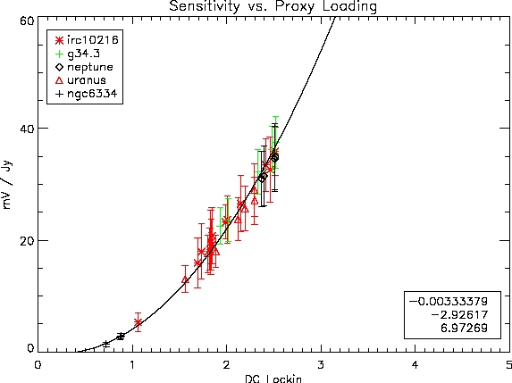
Available as eps and pdf, too. We fit the data to a
quadratic polynomial (which roughly describes the expectation for the
relation). The coefficients of the fit in the order constant,
linear, quadratic are shown.
Simple Application of Flux Calibration
If you're not interested in a very precise flux calibration, then you
can use the following method. This is basically a common
calibration to all the bolometers, without any attempts made to
properly correct for variations in relative calibration or in variation
of the above calibration curve between bolometers. It is good to
10-15%.
The output maps may be calibrated by utilizing the keyword mvperjy in the call to map_ncdf_wrapper.pro. The mvperjy keyword expects the
coefficients of a quadratic fit shown above. For example,
map_ncdf_wrapper,
..., mvperjy = [-0.00333379, -2.92617, 6.97269]
Note that the output map is calibrated in mJy, not Jy. Note also that we
are applying a mean calibration to all the bolometers; for high
precision photometry, we really ought to measure and apply the
relationship bolometer-by-bolometer, but that has not yet been
implemented. Note also that you cannot use map_ncdf_wrapper to create a
coadded map of data taken with a different calibration. This will
be remedied in the near future.
Here are the coefficients, by run (one curve suffices for any given
observing run and chopped/unchopped mode):
JAN, 2003 (UNCHOPPED):
[-46.1937 , 27.1943, -1.63024]
JAN, 2003 (CHOPPED):
[ 18.0 ,
0.0, 0.0]
MAY, 2003 (UNCHOPPED):
[-12.3894 , 7.32377, 1.97081]
MAY, 2003 (CHOPPED):
[ -4.85741 , 2.86853, 0.589577]
FEB, 2004 (UNCHOPPED): [
-0.0909504 , -2.07696, 3.86397]
MAY, 2004 (UNCHOPPED): [
-0.00333379,
-2.92617, 6.97269]
More Correct, Complex Application of Flux Calibration
A more precise application of flux calibration is done as
follows. First, sky noise is used to obtain relative calibration
of different bolometers as a function of "DC Lockin" value.
Second, non-variable pointing sources and known secondary calibrators
are used to simultaneously estimate the dependence of the absolute
calibration the median "DC Lockin" value.
This more complicated flux calibration requires multiple pieces of
information to be saved, so IDL SAV
files are used. Here are the necessary files:
|
Generic
Calibration Files
(needed for all runs, modulo choice of observing band)
|
| 1 mm band camera transmission
spectra |
1mm_spectra.sav |
| 2 mm band camera transmission
spectra |
2mm_spectra.sav |
| Model atmospheric transmission
spectra |
atm_trans.sav |
| Model atmospheric transmission
first derivative with respect to precipitable water vapor spectra |
dTatm_dpw.sav |
Run-Specific Calibration Files
|
October,
2003
|
Relative flux calibration
|
rel_flux_cal_oct03.sav |
Absolute flux calibration
|
flux_cal_oct03.sav |
Revision History
- 2004/01/31 SG
First version
- 2004/02/02 SG
Add details on focusing and determining pointing offset
- 2004/02/04 SG
Add instructions for creating soft links in ~/data to data directories.
- 2004/04/22 SG
Minor updates and corrections.
- 2004/05/21 SG
Note about which version of IDL is necessary to run pipeline
- 2004/05/27 SG
Update links to discussion of focal plane rotation angles.
- 2004/06/20 SG
Provide directions for read-only and writeable CVS archive versions.
- 2004/06/22 SG
Provide May, 2004, calibration information, add link to old manual.
- 2004/07/04 SG
Calibration numbers for all 1.1 mm runs.
- 2004/10/02 SG
Add more details on setting up soft links for data directories.
- 2005/03/18 SG
Update discussion of directories for use of new /bigdisk RAID on puuoo.
- 2005/04/24 SG
Excise IDL journaling from startup code, correct CVSROOT setup for
recent archive changes on prelude.
- 2005/06/04 SG
Update discussion for move of /bigdisk to kilauea.
- 2005/06/27 SG
Update Calibration Information section, add J. Sayers' SAV files.
- 2009/07/10 SG
Make reference to cal_procedure.txt in CVS archive for detailed
calibration instructions.
- 2009/07/15 SG
Update instructions for CVS installation.
- 2009/10/18 SG
Updates to reflect CVS -> SVN conversion (leave SVN installation for
Tom Downes to rewrite).
Update for no longer using source name lists and for update
cleaning_params and mapping_params scheme (always use the same files
for pointing, run-specific files for science fields).
Update for automated setting of dataset and choosing of parameters
files names.
- 2009/12/10 TPD
Updated pipeline installation instructions for SVN, instead of CVS.
Questions or
comments?
Contact the Bolocam support person.